Home | Rambling on Graphs
I am stoked to write this post, about our linear-time algorithm for finding a balanced separator of minor-free graphs, joint with amazing collaborators Édouard Bonnet, Tuukka Korhonen, Jason Li, and Tomáš Masařík. Special thanks to the AlgUW workshop (Bedlewo 09.2025) for giving us an opportunity to get together and solve this problem!
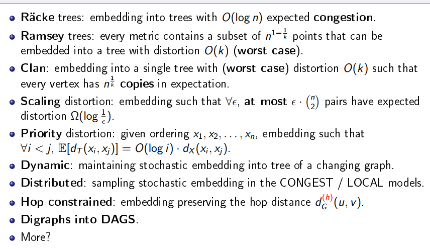
I gave a talk at the Sublinear Graph Simplification workshop at the Simons Institute for Theory of Computing in July 2024. My talk titled “Recent Progress on Euclidean Spanners”, which was my original motivation. However, to fit my talk more to the theme of the workshop, I decided to expand the scope to cover many different types and classes of graphs. Here is a copy of my slides.
In the talk, I posed various questions, and since then, there has been progress on some of them. So I think I should post about these questions and include recent progress on each of them. I wish to see more progress in this space. Without further ado, here they are (refer to my slides for terminology).
Question 1: Show the lightness lower bound \(\Omega(n^{1/k}/\epsilon)\) for \((2k-1)(1+\epsilon)\)-spanners of general graphs (even assuming Erdős’ Girth Conjecture).
The Dagstuhl workshop on “Metric Sketching and Dynamic Algorithms for Geometric and Topological Graphs” I co-organized with Sujoy Bhore, Jie Gao, and Csaba Tóth concluded last week. This is the first Dagstuhl workshop I attended and also happens to be the first I co-organized.
My experience with Dagstuhl was nothing short of amazing. A typical day looks something like this:
- (morning) breakfast, attending a survey talk, group problem-solving for 1.5 hours, and lunch;
- (afternoon) group problem-solving for 1.5 hours, coffee and cake, another hour of group problem-solving, and finally, reporting progress, and dinner;
- (night) night walk or ghost hunting or playing pool, Cheese platter at 9:00 pm, and wine.
A short summary: food + drinks + solving problems. A week like this, away from the end of the semester, was much needed for me.
Dagstuhl provides food, coffee, and cakes. Participants pay for their travel costs (flights, trains, etc.), additional drinks (wine), and room (300 € for 5 days/ person). Organizers get free room.
1. Worshop Structure
As hinted above, we structured our workshop around problem-solving, peppered with invited talks and presentations (from junior participants). I have attended several other problem-solving workshops, and I really love this structure. On a typical day, we had one invited survey talk (about 1.5 hours) in the morning, and the rest of the day, we solved problems in groups.
Here is how it works. Before the workshop, we solicit open problems from participants. We used the coauthor platform to keep track of these problems. (Huge thanks to Erik Demaine for allowing us to use the platform.) On the 1st day of the workshop, problem proposers presented their problems, basically selling them to the workshop audience to attract people to work with the proposer on their problems. After all of these advertisements, we had 3 rounds of voting.
- First round: participants could vote on any problem that they are interested in working on, with no limit on the number of problems one can vote on. After this round, we crossed out problems that received less than 3 votes.
- Second round: Each participant can now vote for up to three problems with 3 different priorities: A, B, and C. Any problem getting less than 1 A vote was crossed out.
- Third round: Each participant can cast exactly 1 vote, and we form groups based on the votes.
Ideally, we want each group to have at least three people and not to be overcrowded (say six people or so). We ended up with six groups (out of 24 people), and every group had at least three people. Participants could also change their group during the week. We stole all the ideas above from various workshops we attended.
One thing that I appreciated from problem-solving workshops (instead of talk-based ones) is that I had an opportunity to work with new collaborators.
2. Invited Talks and Presentations
We invited four survey talks: (1) metric embedding by Arnold Filtser, geometric intersection graphs by Édouard Bonnet, (3) dynamic algorithms in geometry by Wolfgang Mulzer, and (4) routing on plane spanners by Jit Bose.
2.1. Metric Embedding
Arnold surveyed the recent developments of metric embedding into trees and other spin-offs. The talk covered:
- Basic ideas such as padded decomposition, Bartal’s embedding with distortion \(O(\log^2 n)\) and briefly touched upon the embedding with distortion \(O(\log n)\) by Fakcharoenphol, Rao, and Talwar.
- Online metric embeddin, where points arrive online and the decision to embed is irrevocable.
- Embedding into spanning trees: classical results and a recent embedding by Becker, Emek, Ghaffari, and Lenzen using low-diameter decomposition.
- Embedding planar/minor-free graphs into low-treewidth graphs.
And a list of spin-offs that are not covered in detail.
Jonathan Conroy and Arnold Filtser have recently solved the padded decomposition problem for minor-free graphs. Congratulations to both! I wrote about this open problem here in the past.
A \((\beta,\Delta)\)-padded decomposition of \(G = (V,E,w)\) is a stochastic decomposition of \(V\) into a set \(\mathcal{P}\) of clusters of (weak) diameter at most \(\Delta\) such that for every \(v\in V\), the probability that the ball of radius \(\gamma\Delta\) from \(v\) is entirely contained in the cluster of \(v\), denoted by \(\mathcal{P(v)}\), is small. More precisely:
\[\mathrm{Pr}[B_G(v,\gamma \Delta)\subseteq \mathcal{P(v)}] \leq e^{-\beta\gamma} \quad \text{for every }\gamma\ll 1\]
A major open problem was: Can we construct a padded decomposition for \(K_r\)-minor-fre graphs with a padding parameter \(\beta = O(\log r)\)? There has been various partial progress discussed in the previous post for special cases such as bounded genus graphs and bounded treewidth graphs. However for \(K_r\)-minor-fre graphs, the best known bound is \(\beta = O(r)\) also by Arnold. As the title suggested, Jonathan and Arnold have recently solved this problem; the paper will appear in STOC 25.
Many of us know the Four Russians Method, a technique for speeding up Boolean matrix multiplication. The idea is pretty simple, and Wikipedia has a reasonably good summary, which I reproduced here:
The main idea of the method is to partition the matrix into small square blocks of size \(t \times t\) for some parameter \(t\), and to use a lookup table to perform the algorithm quickly within each block. […..] Thus, the overall algorithm may be performed by operating on only \((n/t)^2\) blocks instead of on \(n^2\) matrix cells, where \(n\) is the side length of the matrix. In order to keep the size of the lookup tables (and the time needed to initialize them) sufficiently small, \(t\) is typically chosen to be \(O(\log n)\).
I first learned the Four Russians Method from Jeff Erickson’s note on dynamic programming for the edit distance.
The Four Russians Method was introduced by Arlazarov, Dini\(\check{\mathrm{c}}\), Kronrod, and Farad\(\check{\mathrm{z}}\)ev in this paper about constructing the transitive closure of DAG. The paper is in Russian, and I am not aware of any English translation.
Ben Rozonoyer, a PhD student at UMass, translated the paper to English and gave me permission to publish it in my blog. Check it out here. I worked with Ben on a paper about learning representation of DAGs, and that’s how the four Russian paper interested him. Ben told me that only one of the four authors is ethnically Russian, while ChatGPT insists that all four are.
In computational geometry, dimensionality is a curse. Take the (approximate) nearest neighbor search problem as an example: 1D easy peasy, 2D a whole new level, and \(\log(n)\)-D a completely different world.
Let’s restrict ourselves to low-dimensional spaces. (High-dimensional spaces are too hard for me.) To set the stage for what I will be writing about, let’s ask: Is there any way to reduce a problem in \(\mathrm{R}^d\) for any constant \(d\geq 2\) to 1D? It’s a bold question, and I am definitely NOT the first asker. How about a bolder question: reducing a dynamic problem in \(\mathrm{R}^d\), where points are inserted/deleted dynamically, to a dynamic problem in 1D?
I doubt if we will ever get satisfying answers to these questions. However, locality-sensitive orderings (LSO), the subject of this post, provides a very good answer to both questions: it basically reduces a problem in 2D or above to 1D, even in the dynamic setting. This was eye-opening when I first saw LSO. Over the last few years, I have been trying to understand LSO and extending it to a more general setting of doubling metrics. We have made progress in this direction, which I will also include in this post.
I wrote about multiplicative spanners in the past on this blog. The word “multiplicative” refers to the stretch being multiplicative. This post is devoted to additive spanners, and (a small section) on a recent work with my PhD student An La.
SODA25 list of accepted papers was out. Here I list some papers that are of interest to me, and include arxiv links if available. I will update the arxiv links when they are available in the future.
Here is a simple graph clustering problem. Given a graph \(G = (V,E,w)\) and a parameter \(\Delta > 0\), we want to partition the vertex set \(V\) into clusters such that (1) every cluster has a diameter at most \(\Delta\) and (2) the fraction of edges between clusters is at most \(\beta/\Delta\). Our goal is to minimize \(\beta\) (and thereby minimize the number of edges between clusters).
In a recent preprint with amazing collaborators that I met during a workshop on geometric spanners at the Rényi Institute, we looked into spanners for planar domains such as polygonal domains or polyhedral terrains. One problem arising from this work is constructing a non-Steiner tree cover for tree metrics. So what is it?
Given an edge-weighted tree \(T\) and a subset of terminals \(K\subseteq V(T)\), a non-Steiner tree cover with stretch \(\alpha \geq 1\) is a collection of trees \(\mathcal{T}\) such that:
- [Non-Steiner] every tree \(X\in \mathcal{T}\), \(X\) only contains vertices of \(K\), i.e., \(V(X) = K\).
- [Dominating] for every tree \(X\in \mathcal{T}\), and for every two terminals \(t_1,t_2\in K\), \(\delta_T(t_1,t_2)\leq \delta_X(t_1,t_2)\).
- [Stretch] for every two terminals \(t_1,t_2\in K\), there exists a tree \(X\in\mathcal{T}\) such that \(\delta_X(t_1,t_2)\leq \alpha\cdot \delta_T(t_1,t_2)\).
This post will discuss our recent preprint on tree cover for Euclidean metrics. A line of research that I have been thinking a lot about recently is constructing tree covers for point sets in metric spaces. Intuitively, a tree cover of a point set is a collection of trees such that for any two points in the set, one of the trees preserves their distance up to some stretch factor. More formally, given a set of point \(X\) in a metric space \((M,\delta_M)\), a tree cover of stretch \(\alpha\) for \(P\) is a collection of trees \({\mathcal T}\) such that:
- [Dominating] for every tree \(T\in {\mathcal T}\), \(X\subseteq V(T)\), and for every two points \(x,y\in X\), \(\delta_M(x,y)\leq \delta_T(x,y)\).
- [Stretch] for every tow points \(x,y\in X\), there exists a tree \(T\in{\mathcal T}\) such that \(\delta_T(x,y)\leq \alpha\cdot \delta_M(x,y)\).
The study of tree cover for general graph metrics dates back to 1992, starting from the paper by Awerbuch and Peleg on communication-space trade-off in routing; refer to a short survey on tree conver in the introduction of our paper for more detail.
Tree covers have many algorithmic applications, but my favorite is in constructing an approximate distance oracle, which got me to think more about tree covers in the first place. Say we want to construct an approximate distance oracle for a graph \(G\) with a stretch factor (i.e., distance error) of \(t\), we first construct a tree cover with stretch \(t\) for (the shortest path metric of) \(G\). Then, we construct an exact distance oracle for each tree, that can be reduced to LCA data structure. To answer a distance query between two vertices \(x\) and \(y\), all we have to do is go through each tree in the cover, query the \(x\)-to-\(y\) distance in the tree, and then return the minimum distance among all the trees. The number of trees in the cover will dictate the space of the oracle and the query time; more precisely, \(O(n \lvert{\mathcal T}\rvert)\) space and \(O(\lvert{\mathcal T}\rvert)\) query time. The distance approximation factor is the stretch of the tree cover.
As we have seen, in distance oracles as well as other applications of tree cover, the stretch and the number of trees will be important parameters, and determining the precise trade-off between the two parameters is the most fundamental question.
I am personally interested in constructing tree covers for special metric spaces, such as Euclidean, planar and minor-free, and doubling. In these metrics, the stretch can be made \((1+\epsilon)\) for any \(\epsilon \in (0,1)\), which makes tree covers attractive for various applications. The main question is: Can the number of trees be independent of \(n\), the number of points? It turned out that in all these settings, the number of trees can be made independent of \(n\). (This fact was known for Euclidean metrics a long time ago but only recently known for doulbing, planar and planar metrics. )
Then the next question is: What is the precise dependency on \(\epsilon\) of the number of trees? In the recent preprint, we answered this question.
This post is about my recent preprint with Hsien-Chih Chang and Jie Gao, on the problem of computing diameter of unit disk graphs. (I have not written about my recent papers, and I think I should write more, especially about things that are not included in the papers.)
A unit disk graph with \(n\) vertices is the intersection graph of \(n\) disks on the plane: two vertices have an edge if their two corresponding disks intersect. Here is an example of a unit disk graph; the figure is by David Eppstein on wikipedia:

A unit disk graph could have \(\Omega(n^2)\) edges and hence we often work with its disk representation that only has \(O(n)\) space, hoping to also design algorithms with \(O(n\mathrm{polylog}(n))\) time. For example, single-source shortest path in unit disk graphs can be solved in \(O(n\log n)\) time. Could we design an algorithm for computing diameter with the same running time? This problem currently seems out of reach. An easier problem is to compute the diameter of unit disk graphs in truly subquadratic time. This turns out to be a long-standing open problem.
In the Steiner Point Removal (SPR) problem, we are given an undirected, edge-weighted graph \(G=(V,E,w)\) and a subset of vertices \(K\subseteq V\), called terminals. Non-terminal vertices of \(G\) are called Steiner points. The goal is to find an (edge-weighted) minor \(M\) of \(G\) that only contains the terminal set \(K\) and (approximately) preserves the terminal distances:
\[d_G(t_1,t_2)\leq d_M(t_1,t_2) \leq \alpha \cdot d_G(t_1,t_2)\]
The constant \(\alpha\) is called the distortion of \(M\). We want to construct \(M\) such that \(\alpha\) is as small as possible, ideally \(\alpha = 1\). We call \(M\) the distance preserving minor. Since \(M\) only contains the terminals, by constructing \(M\), we effectively remove Steiner points from \(G\) and hence the name Steiner Point Removal (SPR).
We have the freedom to set the weights of the edges of \(M\) arbitrarily as long as the terminal distances are not contracted. In all known constructions, we often set the weight of each edge \((t_1,t_2) \in E(M)\) to be \(d_G(t_1,t_2)\).
So, what is a minor? The formal definition is: a minor of \(G\) is a graph obtained from \(G\) by deleting vertices, deleting edges, and contracting edges. However, this formal definition is often not useful in constructing a distance-preserving minor. A more intuitive way to think about minor is: every terminal \(t\in K\) has a corresponding subgraph \(H_t\) in \(G\) such that (a) all the graphs \(\{H_t: t\in K\}\) are pairwise vertex-disjoint and (b) there exists an edge \((x,y) \in E(M)\) if there is an edge \((u,v)\) in \(G\) connecting a vertex \(u\in H_x\) and a vertex \(v\in H_y\).

Figure 1: (a) Four terminals in a graph, (b) the disjoint subgraphs associated with each terminal, and (c) a distance-preserving minor. The distortion is \(4/3\) realized by the terminal pair \((t_2,t_3)\).
Why a distance-preserving minor? There are several ways one could construct a graph preserving distances, such as those studied in spanners and emulators literature. However, these graphs often do not preserve structural properties of \(G\): for example, if \(G\) is planar, then these graphs might not be planar. A distance-preserving minor aims to preserve both distances and minor structures: if \(G\) is planar or excludes a fixed minor, then \(M\) also has the same property.
Gupta was the first to study the problem of removing Steiner points in trees: given a set of terminals \(K\) in a tree \(T\), find another tree \(T_K\) spanning the terminals such that the terminals distances in \(T_K\) are approximately the same as the terminal distances in \(T\) up to a small distortion \(\alpha\). Gupta showed that \(\alpha = 8\) is achievable for trees and showed a lower bound \(\alpha\geq 4(1-o(1))\). Chan, Xia, Konjevod, and Richa observed that the tree \(T_K\) in Gupta’s construction is indeed a minor of \(T\), and further improved the lower bound of Gupta to \(\alpha\geq 8(1-o(1))\), matching the upper bound.
Since preserving the minor structure is central in distance-preserving minor, a natural question is:
Question 1: Does every \(K_r\)-minor-free graph for any fixed \(r\) admit a distance-preserving minor with a constant distortion?
This question was raised in the work of Chan, Xia, Konjevod, and Richa as well as an unpublished manuscript by Basu and Gupta.
One could ask same question for general graphs:
Question 2: What is the smallest distortion achieved for the SPR problem in general graphs?
Both questions have attracted significant research interest over the last decade. Until recently, Question 1 remained wide open: no constant upper bound, even for planar graphs. On the other hand, there has been steady progress on the upper bound of Question 2. Filtser showed the distortion \(O(\log \lvert K\rvert)\) for general graphs. However, the best lower bound remains 8 in both cases.
In this post, I am happy to report very recent progress on both questions. Our recent paper resolved Question 1 positively, while Chen and Tan showed the first non-constant lower bound of \(\tilde{\Omega}(\sqrt{\log \lvert K\rvert})\) for Question 2, narrowing the gap with the upper bound of \(O(\log \lvert K\rvert)\) by Filtser. Coincidentally, both papers will appear in SODA 2024.
I attended the workshop in mid-June, and it is one of the best that I’ve ever attended. Thanks to the organizers, Nicole, Zihan, Prantar, and the DIMACS staff, for working on the logistics and booking flights for all the speakers.
I missed several talks, mostly on the 1st and the last day of the workshop, due to travel constraints. The talks I attended were all excellent. Here I give my brief take on each talk, which is likely erroneous and incomplete.
The separator theorem for planar graphs Lipton and Tarjan is the cornerstone of planar graph algorithms: any planar graph of \(n\) vertices can be separated into connected components of size at most \(2(n)/3\) each by removing \(O(\sqrt{n})\) vertices. (An earlier separator theorem by Ungar has a slightly larger size of about \(\sqrt{n}\log^{3/2}n\).) The proof is beautiful but does rquire a non-trivial introduction to planar embedding and its properties, such as the interdigitating tree. My motivation for this post is to look for a proof that does not requires planar embedding. There are many other proofs of the (variants) of the planar separator theorem—see the excellent book chapter by Sariel Har-Peled—but none fits into what I am looking for: a self-contained proof that does not require planar embedding.
To be more precise, I look for a proof that only requires the input graph excluding a fixed minor, \(K_5\) for example in the case of planar graphs. There are two proofs that I particularly like: one by Plotkin, Rao, and Smith [2] and another by Alon, Seymour, and Thomas [1], which work for any graph excluding a fixed minor. I will present both. The central concept is a \(K_h\)-minor model.
\(K_h\)-minor model: a \(K_h\)-minor model of a graph \(G\) is a collection of \(h\) vertex-disjoint connected subgraphs \({\mathcal K} = \{C_1,C_2,\ldots, C_h\}\) of \(G\) such that there is an edge between any two subgraphs. Parameter \(h\) is called the model size.

Figure 1: A graph (left) and its \(K_5\)-minor model (right).
A graph is \(K_h\)-minor-free if it does not have a \(K_h\)-minor model. The Kuratowski’s theorem implies that planar graphs are \(K_5\)-minor-free (and \(K_{3,3}\)-minor-free). Herein we assume that the input graph is \(K_h\)-minor-free, and think of \(h\) as a small constant.
A balanced separator of a graph \(G = (V,E)\) is a subset of vertices \(S\subseteq V\) such that every connected component of \(G\setminus S\) has size at most \(2n/3\). There is nothing special about the constant \(2/3\); any constant smaller than \(1\), for example \(4/5\), works. In some places of this post, we will be handwavy on the constant.
Basic ideas: We will maintain a minor model \({\mathcal K}\) of size \(r\) for some \(r\leq h-1\). At each step, we either increase the model size by \(1\) or find a subset of vertices to add to the separator. This could be achieved, say, by considering a BFS tree rooted at some vertex \(v\), say \(T_v\). There are two cases:
- \(T_v\) has low depth, then we add a subtree of \(T_v\) to the current minor model \({\mathcal K}\). Furthermore, the subtree has a small size since we only need to connect the root \(v\) to at most \(h-1\) other subgraphs, each by a (short) path in \(T_v\).
- \(T_v\) has alarge depth, then some layer of \(T_v\) will have a small size, and we could add this layer to the separator.
In the end, we find either a \(K_h\)-minor model, certifying that the input graph is not \(K_h\)-minor-free, or a balanced separator of small size. We will also add some vertices in the current minor model to the separator and hence, the fact that subgraphs of the minor model have a small size will help.

Figure 2: (a) Found a tree of small depth rooted at a vertex \(v\), then (b) add a new subgraph to the current \(K_3\)-model to obtain a \(K_4\)-model. (c) The tree rooted at \(v\) has large depth, then (d) find a layer \(X\) of small size to add to the separator.
A major subtlety in this basic strategy is to account for the size of the separator in the 2nd case, as the number of iterations could be very large. Two algorithms presented below have very different accounting techniques. Plotkin, Rao, and Smith [2] use charging: they charge the size of the separator (which basically is a BFS layer) to a smaller component after removing the separator, as the algorithm will recurse on the bigger component. Alon, Seymour, and Thomas [1] incorporated the separator directly to the minor model. The end result is that the algorithm by Plotkin, Rao, and Smith produces a larger separator by a factor of \(\sqrt{\log(n)}\) for a constant \(h\).
Merav Parter gave a talk at UMass theory seminar last week titled “Reachability Shortcuts: New Bounds and Algorithms”. In the talk, Merav summarized recent developments in shortcut sets and related concepts. It was amazing to see all the results, and I cannot resist the attempt to share my take here in this blog post.
1. Shortcut set: what is it?
A \(d\)-shortcut set of a directed graph \(G=(V,E)\) is a set of directed edges \(E_H\) such that (i) the graph \(H = (V,E\cup E_H)\) has the same transitive closure as \(G\) and (ii) for every \(u\not=v\in V\), if \(v\) is reachable from \(u\), then there is directed \(u\)-to-\(v\) path of at most \(d\) edges (a.k.a. hops).

Figure: Adding two shortcuts (the red dashed edges) reduces the hop distance from \(u\) to \(v\) to 4. For a shortcut set of linear size, DAG is the most difficult instance: one can shortcut any strongly connected graph to diameter \(2\) by \(n-1\) edges.
The shortcut set problem was introduced by Thorup. The main goal is to understand the trade-off between the hop diameter \(d\) and the size of the shortcut set \(E_H\). The most well-studied regime is fixing \(\lvert E_H\rvert = \tilde{O}(n)\), and then minimizing \(d\). (Here, \(n\) is the number of vertices.) We will call this special regime the shortcut set problem.
This post describes a simple linear time algorithm by Halperin-Zwick [6] for constructing a \((2k-1)\)-spanner of unweighted graphs for any given integer \(k\geq 1\). The spanner has \(O(n^{1+1/k})\) edges and hence is sparse. When \(k = \log n\), it only has \(O(n)\) edges. This sparsity makes spanners an important object in many applications.
This post was inspired by my past attempt to track down the detail of the Halperin-Zwick algorithm. Halperin and Zwick never published their algorithm, and all papers I am aware of cite their unpublished manuscript [6]. The algorithm by Halperin-Zwick is a simple modification of an earlier algorithm by Pelege and Schäffer [8], which, according to Uri Zwick, is the reason why they did not publish their result. The spanner by Pelege and Schäffer [8] has stretch \(4k-3\) for the same sparsity. The idea of Halperin-Zwick algorithm was given as Exercise 3 in Chapter 16 of the book by Peleg [7].
First, let’s define spanners. Graphs in this post are connected.
\(t\)-Spanner: Given a graph \(G\), a \(t\)-spanner is a subgraph of \(G\), denoted by \(H\), such that for every two vertices \(u,v\in V(G)\):
\[d_H(u,v)\leq t\cdot d_G(u,v)\]
Here \(d_H\) and \(d_G\) denote the graph distances in \(H\) and in \(G\), respectively. Graph \(G\) could be weighted or unweighted; we only consider unweighted graphs in this post. The distance constraint on \(H\) implies that \(H\) is connected and spanning.
Parameter \(t\) is called the stretch of the spanner. We often construct a spanner with an odd stretch: \(t = 2k-1\) for some integer \(k\geq 1\). Why not even stretches? Short answer: there is no gain in terms of the worst case bounds for even stretch [1].
Over the past two years or so, I have been thinking about a cute problem, which turned out to be much more useful to my research than I initially thought. Here it is:
Tree Shortcutting Problem: Given an edge-weighted tree \(T\), add (weighted) edges to \(T\), called shortcuts, to get a graph \(K\) such that:
- \(d_K(u,v) = d_T(u,v)~\quad \forall u,v\in V(T)\). That is, \(K\) preserves distances in \(T\).
- For every \(u,v\in V(T)\), there exists a shortest path from \(u\) to \(v\) in \(K\) containing at most \(k\) edges for some \(k\geq 2\).
The goal is to minimize the product \(k \cdot \mathrm{tw}(K)\), where \(\mathrm{tw}(K)\) is the treewidth of \(K\).
Planar graphs are sparse: any planar graph with \(n\) vertices has at most \(3n-6\) edges. A simple corollary of this sparsity is that planar graphs are \(6\)-colorable. There is simple and beautiful proof based on the Euler formula, which can easily be exteded to bounded genus graphs, a more general case: any graph embedddable in orientable surfaces of genus \(g\) with \(n\) vertices has at most \(3n + 6g-6\) edges.
How’s about the number of edges of \(K_r\)-minor-free graphs? This is a very challenging question. A reasonable speculation is \(O(r)\cdot n\): a disjoint union of \(n/(r-1)\) copies of \(K_{r-1}\) excludes a \(K_r\) minor and has \(\Theta(r)\cdot n\) edges. But this isn’t the case. And surprisingly, the correct bound is \(O(r\sqrt{\log r})n\), which will be the topic of this post.
Theorem 1: Any \(K_r\)-minor-free graphs with \(n\) vertices has at most \(O(r\sqrt{\log r})\cdot n\) edges.